By iterating through each value in noise_range and adding noise to each data point’s price feature, the code generates multiple data points with different levels of noise. This process results in more labeled data points for the machine learning model to learn from and improves the model’s accuracy.
noise_range is a list of standard deviation values for generating different levels of noise. It could be any list of values to add different levels of noise to the data points:
- for noise in noise_range creates a loop that iterates through each value in the noise_range list.
- new_row = row.copy() creates a copy of the original data point (i.e., row).
- new_row[“price”] = add_noise(row[“price”], noise) adds noise to the copied data point’s price feature using the add_noise() function. The add_noise() function adds random noise to each data point based on the standard deviation provided in the noise variable.
- augmented_data.append(new_row) appends the newly generated data point to the augmented_data list. The augmented_data list contains all the newly generated data points for all levels of noise in the noise_range list.
Similarly, let’s define another data augmentation scale function:
def scale(x, factor):
return x * factor
scale_range = [0.5, 0.75, 1.25, 1.5]
The range of parameters for scale_range is defined, and for each available data point, it generates multiple augmented data points with different parameter values:
for scale_factor in scale_range:
new_row = row.copy()
new_row[“price”] = scale(row[“price”], scale_factor)
augmented_data.append(new_row)
In this code snippet, we’re utilizing data augmentation to generate augmented data by applying scaling to the price feature. For each scale factor within the specified scale_range, we duplicate the current data row by creating a copy of it using row.copy(). Then, we apply scaling to the price feature using scale_factor, effectively modifying the price values while preserving the data’s relationships.
Finally, the augmented row is added to the list of augmented data stored in the augmented_data list. This approach empowers us to explore how varying scales affect the price feature and enrich our dataset with diverse instances for improved model training and testing:
# Combine the original data and the augmented data
combined_data = pd.concat([df, pd.DataFrame(augmented_data)])
Here’s the augmented data:
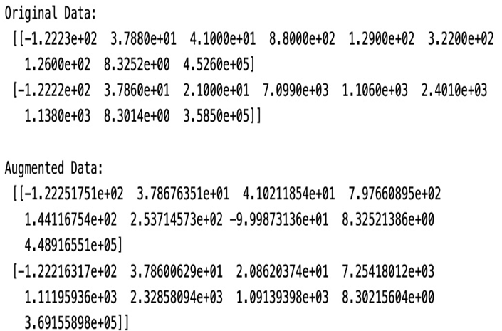
Figure 3.5 – Original data and augmented data
The code then combines the original labeled data with the augmented data, splits it into training and testing sets, trains a linear regression model on the combined data, and evaluates the model’s performance on the test set using mean squared error as the evaluation metric:
# Split the data into training and testing sets
X = combined_data.drop(“price”, axis=1)
y = combined_data[“price”]
X_train, X_test, y_train, y_test = train_test_split(X, y, \
test_size=0.2, random_state=42)
# Train a linear regression model
model = LinearRegression()
model.fit(X_train, y_train)
# Evaluate the model
y_pred = model.predict(X_test)
mse = mean_squared_error(y_test, y_pred)
print(“Mean Squared Error:”, mse)
By iterating through each value in noise_range and adding noise to each available data point, it generates multiple augmented data points with different levels of noise. This process results in more labeled data points for the machine learning model to learn from and improves the model’s accuracy. Similarly, scale factor and rotation degree are used to generate labeled data using data augmentation to predict house prices using regression.
In this section, we have seen how to generate the augmented data using noise and scale techniques for regression. Now, let’s see how we can use the K-means clustering unsupervised learning method to label the house price data.